
JLP Delta-Neutral: a hedged Jupiter liquidity strategy
Abstract
This paper describes a market-neutral yield strategy on Jupiter Perps, Solana's largest perpetuals venue. The strategy holds JLP - the venue's liquidity token - collects the fee stream it earns, and removes the token's crypto exposure with a continuously rebalanced hedge. The result is a return stream driven by trading-fee revenue rather than market direction.
Contents
1. Introduction
1.1 What JLP is
Jupiter Perps is Solana's largest perpetuals venue. Its liquidity pool - tokenized as JLP - is the house side of every trade: the pool holds a basket of SOL/ETH/BTC plus stables, lends that inventory to leveraged traders, and earns fees for it. JLP's virtual price (pool NAV / supply) compounds those earnings automatically.
1.2 Why Jupiter Perps
Jupiter is the #1 perpetuals DEX on Solana by volume and TVL, and one of the largest on-chain derivatives venues overall. At its peak the JLP pool held over $2B in assets (~$830M today), and the venue has operated through multiple full market cycles without a solvency incident. We therefore treat Jupiter as a comparatively low counterparty risk among yield sources of this size - the protocol is battle-tested, fully on-chain and independently verifiable at any moment.
1.3 Where the yield comes from
Traders pay the pool at every step of their trade: a fee to open a position, a fee to close it, and an hourly borrow fee for the leverage while the position stays open. On top of the fee stream, the pool is the counterparty of every trade - so aggregate trader losses accrue to it as well. 75% of venue fees flow to JLP holders, embedded directly into the token price.
1.4 The need for hedging
Raw JLP is a leveraged-fee business wrapped in a crypto index: its basket exposure dominates short-term returns and can erase months of fee income in a drawdown. Isolating the fee business from the index is the entire point of this strategy - and doing it well is a data and execution problem, which is where the rest of this paper lives.
2. Strategy mechanics
2.1 What we do
Raw JLP carries the crypto exposure of its basket. The strategy strips that exposure away and keeps the yield: we hedge out the SOL/BTC/ETH delta, apply moderate leverage to the position, execute rebalancing with tight cost control, route the hedge to whichever venue makes it cheapest at the moment, and layer additional yield sources on top of the core position.
2.2 Delta methodology
The key subtlety of hedging JLP is that we hedge the risk traders transfer to the pool, not simply the assets the pool holds. The pool is the counterparty of every open position: a trader's long takes exposure away from liquidity providers, a trader's short hands exposure back. Hedging the raw basket would therefore be wrong whenever open interest is non-zero - and it almost always is.
For each volatile asset the per-JLP hedge target is the pool's trader-adjusted exposure, normalized by supply:
2.2.1 How we verified the deltas are right
We ran the simplest possible test: an idealized simulation - a continuous hedge driven purely by formula (1) over 2.5 months of pool data, no cost optimizations, no execution logic. It is a test of the delta computation, not a P&L projection.
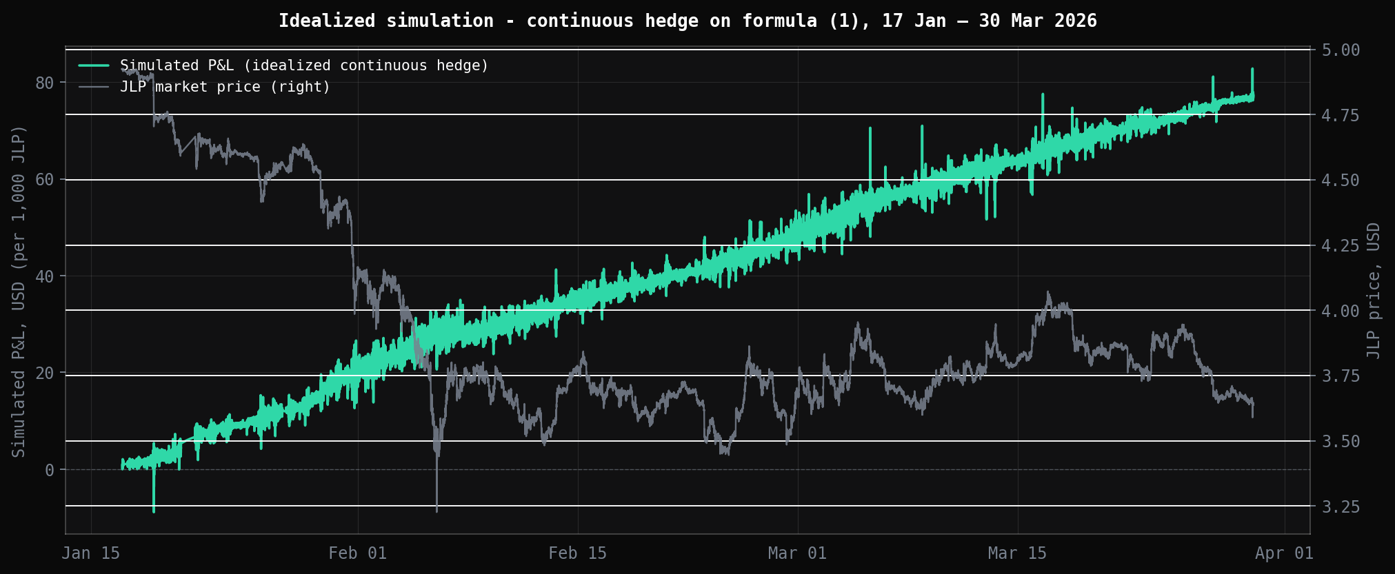
JLP fell 26% over the window - and the hedged P&L grew steadily, with no imprint of the price path. If the deltas were computed wrong, a trend of that size would leak straight into the P&L; the clean line is the verification.
2.3 Hedging venues
We recompute hedge targets from the pool's on-chain state continuously and maintain offsetting positions across two venues - Hyperliquid and Jupiter Lend - keeping the strategy's net crypto delta pinned near zero while the fee stream accrues. Venue choice per leg is a cost decision (funding, borrow rates, margin efficiency), re-evaluated as conditions move.
2.4 Rebalancing
There are three broad ways to keep a hedge aligned with a moving target: rebalance on a clock (time-based), rebalance when the delta drifts past a bound (threshold-based), or blend the two. We researched each family on our pool data - time grids from minutes to daily, a range of drift bounds, and mixed schemes - and settled on threshold-based rebalancing: the book trades only when a leg's deviation from its ideal exceeds X% (the exact bound is proprietary). This concentrates trading exactly where it pays for itself: quiet markets generate near-zero costs, trend days trigger the hedge precisely when exposure builds.
2.5 Execution
Execution quality is where the threshold policy is won or lost, and each venue gets its own machinery. On Jupiter Lend, the swap legs are routed through the execution infrastructure of our MEV desk - the same low-latency stack that competes in open-venue auctions - which keeps swap slippage tight. On Hyperliquid the rebalancer works with resting limit orders rather than crossing the spread as a taker; at low latency the book comes to us, converting taker fees plus impact into maker-side fills.
3. Backtesting methodology
3.1 Data
The backtest runs entirely on data we collect ourselves - no third-party datasets or aggregators anywhere in the path.
- Source. Our own pipeline reads the pool's state directly from the chain, continuously.
- Captured per snapshot: pool composition and JLP supply; the contract's official AUM; trader open interest (long and short) per asset; oracle prices; JLP premium/discount to NAV.
- Hedge-side inputs. Funding histories from the hedge venues themselves - actual historical hourly rates, not period averages; borrow and deposit rates from on-chain lending markets.
- Validation. Every snapshot passes sanity checks before entering the dataset; invalid snapshots are flagged and excluded - never silently patched or interpolated.
- Continuous reconciliation. The assembled state is checked against the pool contract's own accounting on every snapshot, so a decoding or methodology error cannot quietly poison the history.
- One pipeline. The same data path feeds the backtest and production - there is no simulation-only data.
3.2 Assumptions
Assumptions are chosen to under-claim rather than flatter:
- Execution cost. Every rebalancing trade is charged a taker-cost assumption calibrated to realized execution - conservative, given that live Hyperliquid rebalancing works with maker-side fills.
- DEX swap costs. The swap legs (entering, exiting and resizing the on-chain side of the position) are charged swap fees and price impact - execution costs cover both perp trades and DEX swaps, not perps alone.
- No intra-snapshot trading. Price moves between consecutive snapshots are not traded - the simulation cannot react faster than the data it stands on.
- No look-ahead. Every decision at time t uses only data available at t.
- Reporting discipline. Results use robust window-averaged estimators rather than endpoint deltas; minute-level series are treated as noise-bearing rather than signal.
3.3 Model
The backtest is produced by the same research function that designed the strategy - there is no separate backtest codebase to drift away from production. It simulates the full book in one pass: the JLP position, every hedge leg, funding flows, execution costs and the cost of leverage, with threshold-based rebalancing identical to the production policy (section 2.4). Funding for the hedge legs is modeled from the venues' own rate histories.
The configuration itself is the product of a dedicated research effort: we compared hedging venues and leverage structures across dozens of configurations, and evaluated time-based, threshold and mixed rebalancing regimes inside this same framework. The deployed setup won on realized cost-risk balance, not on the prettiest curve.
3.4 Validation: how we know the backtest is right
A backtest is easy to make look good; the honest test is a head-on collision with reality. Because the model and production share one data pipeline and one codebase, we can replay the exact live window through the backtest and lay the two curves on top of each other - and we do this continuously, not once.
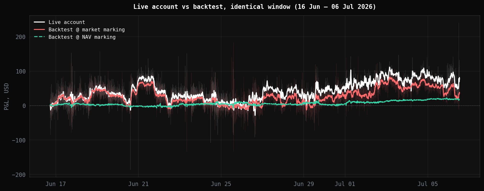
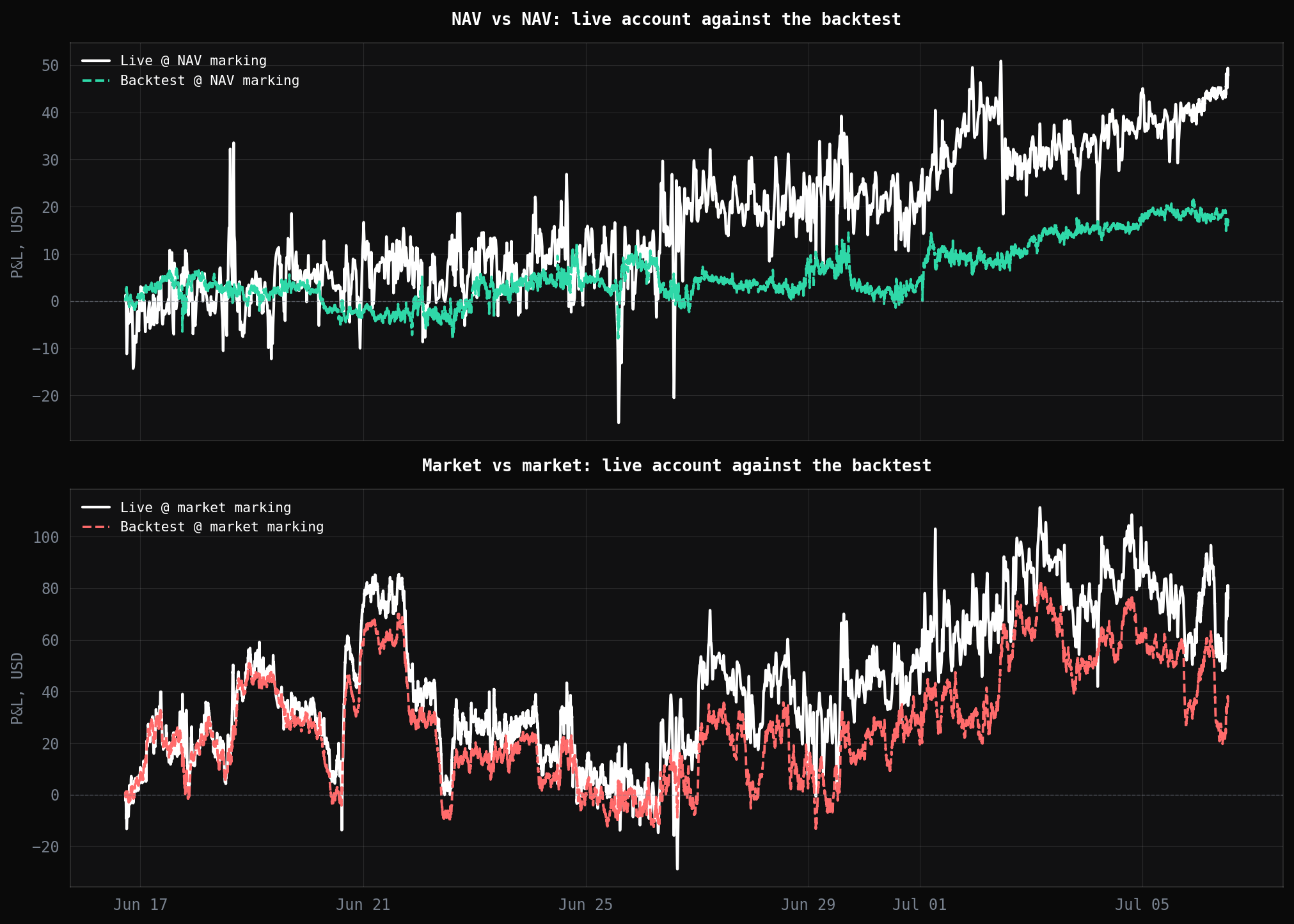
Over the 20-day window the live account and the backtest produced almost the same P&L in both markings, with the live account slightly ahead - expected, since the model's cost assumptions are deliberately conservative. The remaining difference is small and does not grow over time. Section 4 looks at the two markings in detail.
3.5 Final backtest
The headline artifact: the deployed configuration - full costs, funding, leverage and the production rebalancing policy - over 2.5 months of pool data, marked at NAV.
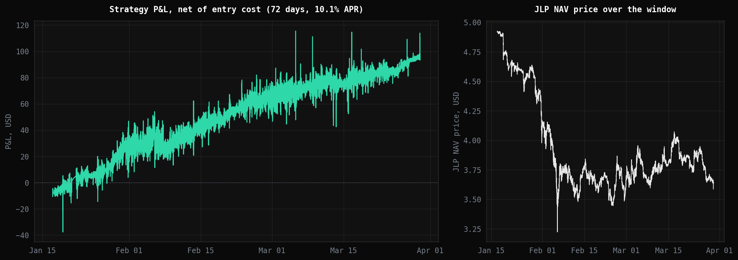
| Metric | Value |
|---|---|
| APR, gross of entry (annualized) | 11.2% |
| APR, net of entry (annualized) | 10.1% |
| Sharpe (daily obs, annualized) | 5.0 |
| Max drawdown | −0.5% of equity |
| Marking | NAV (see section 4 for why) |
4. Live track record & model coherence
4.1 The marking problem: NAV vs market price
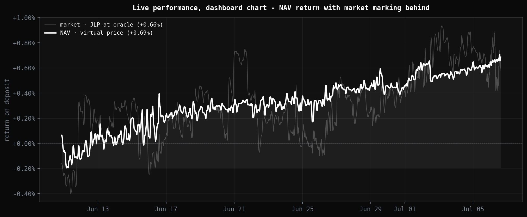
JLP has two prices. The NAV (virtual) price is what the pool contract computes: assets under management divided by supply - the economic value of the claim. The market price is whatever the secondary market pays at this second, and it wanders around NAV in a premium/discount band. The strategy's hedge neutralizes the basket - but nothing can neutralize the premium/discount without giving up the yield, so a market-marked P&L inherits its noise.
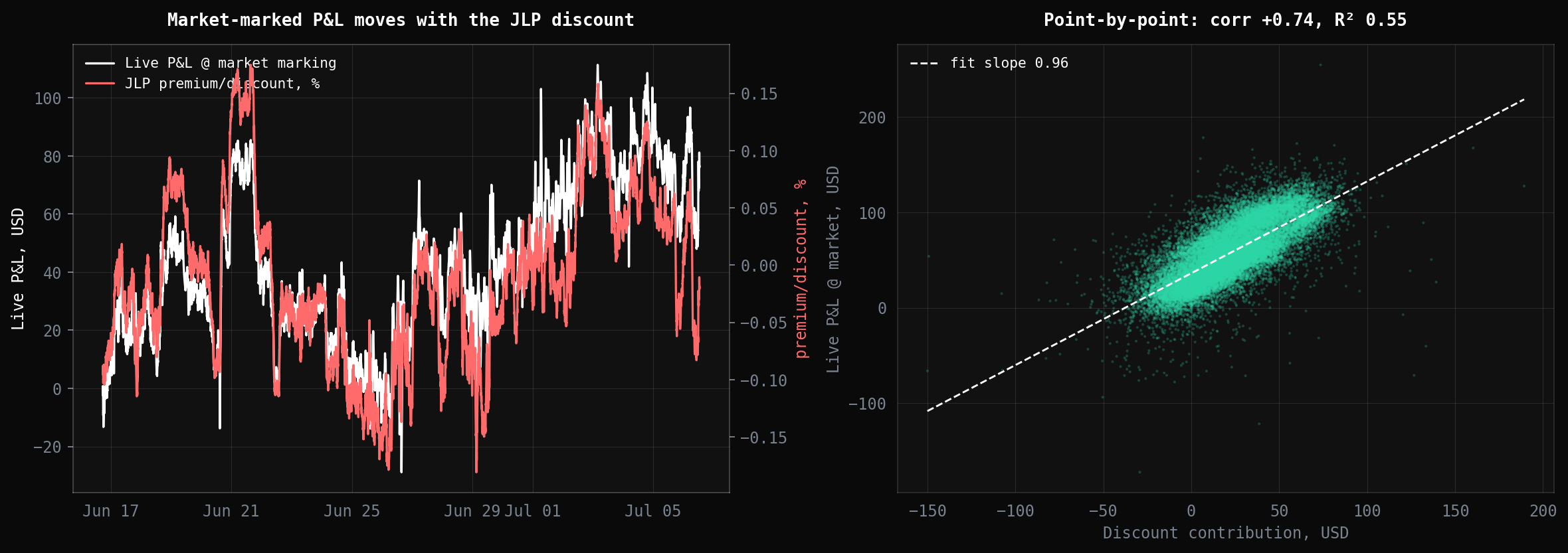
The relationship is direct: the discount passes through into market-marked P&L almost one-for-one and explains most of its short-horizon variance. Short-horizon market-marked P&L is mostly discount noise, not strategy economics.
Why NAV is the honest mark. The discount is transient: on our telemetry the premium touched zero-or-positive territory on 99% of live days - so a NAV-based exit is realizable essentially every day, and marking the smart contract's share price at NAV is fair to investors regardless of when they enter or exit. Marking at market would instead expose every deposit and withdrawal to a random ±1% swing decided by that second's discount.
4.2 Entry cost
What is real, and what we account for separately, is the one-off cost of entering the position: swapping into JLP and standing up the hedge legs costs swap fees plus price impact - about 0.2% of gross position size in the backtest's conservative estimate. Because it is paid once, it amortizes over the holding period: annualized returns are therefore most informative gross of entry cost, with entry shown separately (section 4.5) - on any horizon beyond a few weeks the difference fades into noise.
4.3 Backtest vs live, matched markings
The direct check of model coherence: the same window, marking against marking - live NAV P&L against the backtest at NAV, and live market P&L against the backtest at market. Both pairs track each other within basis noise.
4.4 Live P&L in both markings
| NAV marking | Market marking | |
|---|---|---|
| APR, gross of entry (annualized) | ~12.6% | ~12.2% |
| Sharpe (annualized) | 5.5 | 2.4 |
| Volatility (annualized) | 2.3% | 5.0% |
| Max drawdown | −0.25% | −0.85% |
The NAV series is the strategy; the market series is the strategy plus discount weather - more noise around the same path, which is the visual version of section 4.1.
4.5 Headline figures
| Figure | Value |
|---|---|
| Live pilot APR, gross of entry (NAV) | ~12.6% |
| Final backtest APR, gross of entry | 11.2% |
| Final backtest APR, net of entry | 10.1% |
| Final backtest Sharpe | 5.0 |
| Entry cost | ~0.2% of gross |
5. Infrastructure & custody
5.1 The design goal
The architecture is built so that the client does not carry the failure of any single party - including us. Funds sit in Cobo institutional MPC custody; investor rights are recorded on-chain through a Voltr vault; our systems can manage positions but cannot walk away with assets. Each component is chosen so that its compromise degrades service, not principal - the specific failure modes are traced one by one in section 6. Live positions and NAV are published on the dashboard, so verification never depends on trust.
5.2 Why Voltr
Voltr is vault infrastructure on Solana: it issues LP tokens to the client and enforces deposit, withdrawal and fee mechanics on-chain (vault account, security & audits). The critical property: client money is not stored in Voltr. The vault is the accounting and rights layer - it records who is owed what and lets investors transact self-custodially - while the working capital itself sits in Cobo custody. Voltr's failure domain is bookkeeping, not assets.
5.3 Why Cobo
Cobo is an institutional digital-asset custodian serving exchanges, funds and market makers since 2017. Client capital sits in MPC custody: no single party ever holds the full key, and every transaction must be co-signed under custody-level policies - whitelists, limits and approvals that sit below any code we write. Accounts are segregated per strategy.
5.4 Accounts for larger clients ($100k+)
Clients above $100k do not join the pooled vault at all. Each receives a dedicated, segregated Cobo custody account for their capital - their funds never touch the shared vault infrastructure. What we receive is strictly a management mandate: permission to run the strategy's trades inside the client's own account, under the account's transaction policies. Our operational compromise - or even our disappearance - does not cut the client off from their funds.
5.5 Pooled vault for smaller clients (<$100k)
Clients below $100k enter through the shared Voltr vault. The vault's share price is posted by us and is computed from the strategy's NAV - JLP at its virtual price plus hedge legs - for the reasons established in section 4.1: NAV marking keeps entries and exits fair regardless of the secondary-market discount of the moment. Fee mechanics (performance with high-water mark, management) are enforced by the vault program on-chain.
6. Risk framework
6.1 External smart contracts (Jupiter Perps, Jupiter Lend, Hyperliquid)
The strategy's working capital lives inside third-party protocols: JLP itself (Jupiter Perps), the lending market used by the hedge (Jupiter Lend), and the perp venue (Hyperliquid). An exploit of any of them can impair the corresponding leg up to its full size. Mitigation is selection and sizing, not hope: all three are among the largest, longest-running venues of their class, and exposure per venue is bounded by the strategy's construction. This residual risk is inherent to the yield source and cannot be structured away.
6.2 Voltr compromise - funds are not there
A Voltr smart-contract exploit does not reach client funds, because funds are not stored in the vault (section 5.2): the vault records investor claims while capital sits in Cobo custody. If the vault were compromised, the loss would be the bookkeeping rail, not the assets - and we would settle investor balances manually, paying out directly to client wallets from custody based on the on-chain record of deposits.
6.3 Cobo compromise - funds freeze, not vanish
Cobo custody is MPC/TSS: the signing key exists only as distributed shards, and a transaction requires a threshold of parties to co-sign. A compromise of Cobo's infrastructure therefore does not hand anyone a key to move funds - what it does is halt co-signing. The realistic failure mode is a freeze: assets stay where they are, immovable, until the custodian restores its side of the ceremony. Unpleasant - positions cannot be rebalanced during the freeze - but principal is not lost.
6.4 Off-chain custody & MPC risk
The hedge leg runs on external venues with assets in institutional MPC/TSS custody (Cobo). This portion is not secured by the on-chain vault: compromise or collusion of the MPC signer set, or failure of the custodian or venues, could lead to loss of the off-chain capital. Custody-layer whitelists, limits and approvals bound what any single compromised participant can do.
6.5 Our servers
The trading and data infrastructure runs on AWS. A compromise of these servers mirrors the Cobo case: the machines hold no keys capable of withdrawing client funds - they compute targets and submit proposals that are still subject to the custody layer's policies and co-signing. The realistic damage is operational (halted or degraded rebalancing), not loss of principal.
6.6 Market and other risks
- Market & hedging risk. JLP and the hedge instruments can move sharply and correlate under stress. Hedges may be ineffective or delayed due to liquidity constraints, slippage, funding/borrow costs, or extreme conditions; leveraged perp and lending positions carry liquidation risk.
- Asset risk. All tokens involved (including JLP, USDC and the hedged assets) carry their own market, depeg and counterparty risks.
- Operational risk. Outages, RPC/network issues, or software/monitoring errors may impair execution and rebalancing. Outcomes can vary materially, including adverse results.
- Liquidity risk. Under stressed conditions withdrawals may take longer while capital is unwound from strategy positions.
7. Capacity
Capacity is bounded by four independent constraints; the strategy's ceiling is the tightest of them. Our internal capacity study analyzed each (figures below are from that study's market snapshot and are being refreshed for current venues and pool size):
| Constraint | Mechanism | Est. ceiling |
|---|---|---|
| Fee revenue dilution | strategy AUM earns a share of a finite fee pool; yield floor sets max share | ~$500M |
| Perp hedge slippage | rebalancing flow vs order-book depth; costs grow superlinearly with size | ~$100M |
| DEX swap slippage | entering/unwinding the on-chain leg through AMM liquidity | ~$50M |
| Open-interest share | hedge position capped at a prudent share of venue OI per asset | ~$100M |
The binding constraint in the study was DEX swap liquidity at roughly $50M - a worst-case, single-order estimate; staged execution raises it. Two structural notes: capacity scales with the venues (JLP pool size, hedge-venue depth and OI all grew through past cycles), and constraints bind gradually - costs rise before capacity is reached, so the practical policy is monitored soft limits, not a cliff.
8. Backtest input data
Every number in this paper traces to data an outside party can re-derive. The input dataset behind the 2.5-month backtest window (17 Jan - 30 Mar 2026) is available for download: pool state snapshots (contract AUM, JLP supply, NAV price), trader open interest per asset, oracle prices, and the funding and borrow rate histories used for the hedge legs. Together with formula (1) it is sufficient to reproduce the idealized simulation of Figure 1 independently - in a spreadsheet, if desired.
Download: jlp-backtest-inputs.zip (~12 MB, CSV). The codebase - execution logic, thresholds and optimizations - is not shared: it is the strategy's alpha.
9. Further reading
- Jupiter Perps - the venue; JLP pool mechanics and stats
- Jupiter Lend and Hyperliquid - hedge venues
- Voltr - vault infrastructure (security & audits); Cobo - MPC custody
- On-chain: JLP pool · strategy vault
- Live dashboard - minute-level NAV, allocations, position
Working paper v1.0 · 2026-07-06